🕔 Modelling Time Series
 Photo by Maddi Bazzocco on Unsplash
Introduction
In this module we will look at modelling of time series. We will start with the simplest of expoential models and go all the way through ARIMA and forecasting with Prophet.
First, some terminology!
Additive and Multiplicative Time Series Models
Additive Time Series can be represented as:
\[ Y_t = S_t + T_t + ϵ_t \]
Multiplicative Time Series can be described as:
\[ Y_t = S_t × T_t × ϵ_t \]
Let us consider a Multiplicative Time Series, pertaining to sales of souvenirs at beaches in Australia: The time series looks like this:
Note that along with the trend, the amplitude of both seasonal and noise components are also increasing in a multiplicative here !! A multiplicative time
series can be converted to additive by taking a log of the time series.
Stationarity
A time series is said to be stationary if it holds the following conditions true:
- The mean value of time-series is constant over time, which implies, the trend component is nullified/constant.
- The variance does not increase over time.
- Seasonality effect is minimal.
This means it is devoid of trend or seasonal patterns, which makes it looks like a random white noise irrespective of the observed time interval.( i.e. self-similar and fractal)
A Bit of Forecasting?
We are always interested in the future. We will do this in three ways:
- use Simple Exponential Smoothing
- use a package called
forecastto fit an ARIMA (Autoregressive Moving Average Integrated Model) model to the data and make predictions for weekly sales; - And do the same using a package called
prophet.
Forecasting using Exponential Smoothing
For example, the file contains total annual rainfall in inches for London, from 1813-1912 (original data from Hipel and McLeod, 1994).
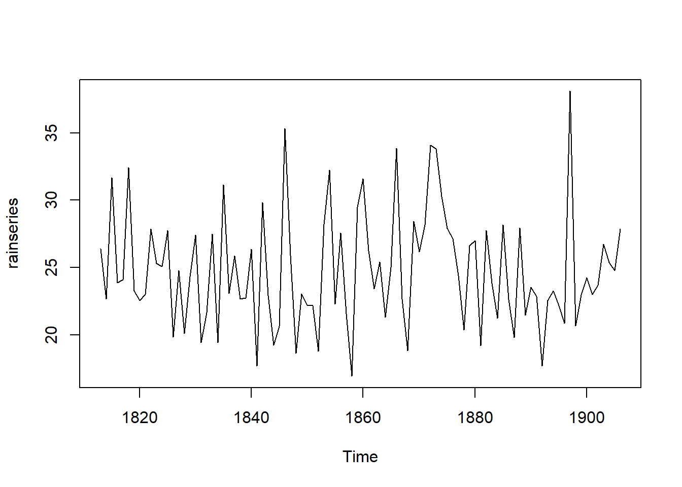
There is a nearly constant value of about 25 around which there are random fluctuations and it seems to be an additive model. How can we make forecasts with this time series?
A deliberate detour:
Let’s see some quick notation to aid understanding: Much of smoothing is based on the high school concept of a straight line, $ y = m * x + c$.
In the following, we choose to describe the models with:
- \(y\) : the actual values in the time series
- \(\hat y\) : our predictions from whichever model we create
- \(l\) : a level or mean as forecast;
- \(b\) : a trend variable; akin to the slope in the straight line equation;
- \(s\) : seasonal component of the time series. Note that this is a set of values that stretch over one cycle of the time series.
In Exponential Smoothing and Forecasting, we make three models of increasing complexity:
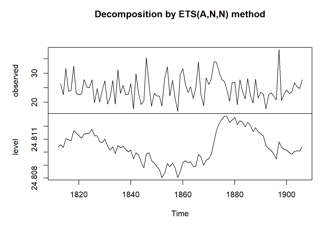
Simple Exponential Model: Here we deal only with the mean or level aspect of the (decomposed) time series and make predictions with that.
Holt Model: Here we use the
leveland thetrendfrom the decomposed time series for predictionsHolt-Winters Model: Here we use the
level, thetrend, and theseasonalcomponent from the decomposed time series for predictions.
Simple Smoothing is smoothing based forecasting using just the level ( i.e. mean) of the Time Series to make forecasts.
Double exponential smoothing, or Holt Smoothing Model, is just exponential smoothing applied to both level and trend.
The idea behind triple exponential smoothing, or the Holt-Winters Smoothing Model, is to apply exponential smoothing to the seasonal components in addition to level and trend.
What does “Exponential” mean?
All three models use memory: at each time instant in the Time Series, a set of past values, along with the present sample is used to make a prediction of the relevant parameter ( level / slope / seasonal). These are then added together to make the forecast.
The memory in each case controlled by a parameter: alpha for the estimate of the level
beta for the slope estimate, and gamma for the seasonal component estimate at the current time point. All these parameters are between 0 and 1. The model takes a weighted average of past values of each parameter. The weights are derived in the form of \(\alpha(1-\alpha)^i\), where \(i\) defines how old the sample is compared to the present one, thus forming a set of weights that decrease exponentially with
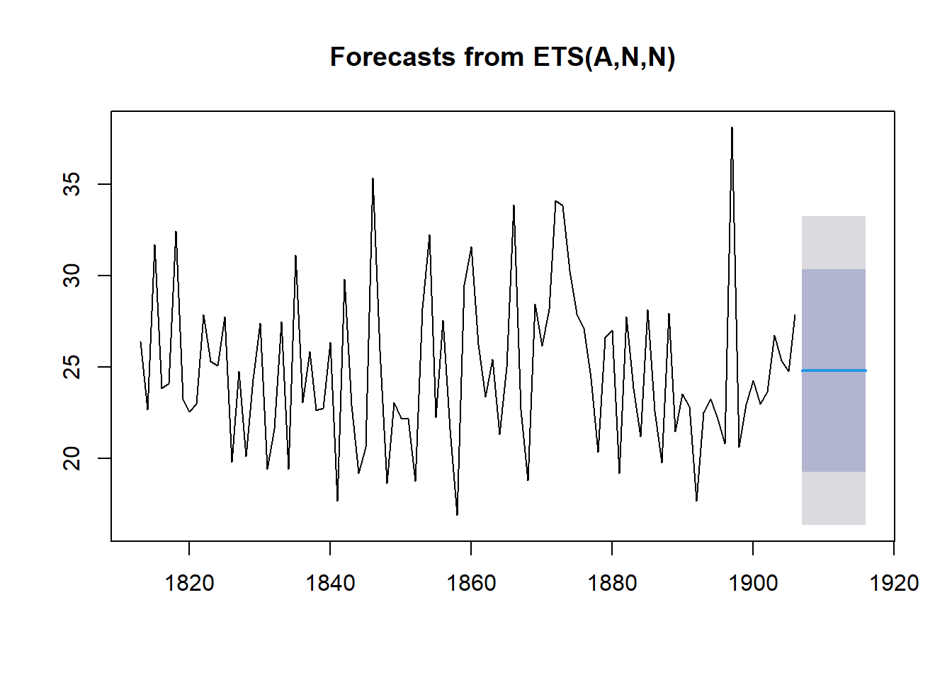
To make forecasts using simple exponential smoothing in R, we can use the HoltWinters() function in R, or the forecast::ets() function from forecasts. This latter function s more powerful.
## function (x, alpha = NULL, beta = NULL, gamma = NULL, seasonal = c("additive",
##     "multiplicative"), start.periods = 2, l.start = NULL, b.start = NULL,
##     s.start = NULL, optim.start = c(alpha = 0.3, beta = 0.1,
##         gamma = 0.1), optim.control = list())
## NULL
## function (y, model = "ZZZ", damped = NULL, alpha = NULL, beta = NULL,
## gamma = NULL, phi = NULL, additive.only = FALSE, lambda = NULL,
## biasadj = FALSE, lower = c(rep(1e-04, 3), 0.8), upper = c(rep(0.9999,
## 3), 0.98), opt.crit = c("lik", "amse", "mse", "sigma",
## "mae"), nmse = 3, bounds = c("both", "usual", "admissible"),
## ic = c("aicc", "aic", "bic"), restrict = TRUE, allow.multiplicative.trend = FALSE,
## use.initial.values = FALSE, na.action = c("na.contiguous",
## "na.interp", "na.fail"), ...)
## NULLTo use HoltWinters() for simple exponential smoothing, we need to
set the parameters beta=FALSE and gamma=FALSE in the
HoltWinters() function (the beta and gamma parameters are used for
double exponential smoothing, or triple exponential smoothing.
To use forecast::ets, we set the model argument to “ANN”, “AAN”, and “AAA” respectively for each of the three smoothing models.
Note: The HoltWinters() function returns a list variable, that contains
several named elements.
ARIMA
We can also use past trends and seasonality in the data to make predictions about the future using the forecast package. Here we use an auto ARIMA model to guess at the trend in the time series. Then we use that model to forecast a few periods into the future.
Mathematically an ARIMA model can be shown as follows:
We will use the familiar Walmart Sales dataset, and try to predict weekly sales for one of the Departments.
## Time Series:
## Start = c(2010, 1)
## End = c(2012, 52)
## Frequency = 52
##   [1] 106690.06 111390.36 107952.07 103652.58 112807.75 112048.41 117716.13
##   [8] 113117.35 111466.37 116770.82 126341.84 110204.77 107648.14 125592.28
##  [15] 120247.90 120036.99 121902.19 133056.97 131995.00 134118.05 120172.47
##  [22] 124821.44 126241.20 121386.73 116256.35 108781.57 131128.96 131288.83
##  [29] 124601.48 117929.58 124220.10 125027.49 124372.90 114702.69 113009.41
##  [36] 120764.22 123510.99 110052.15 105793.40 110332.92 110209.31 107544.02
##  [43] 106015.41 100834.31 111384.36 116521.67 121695.13  93676.95 107317.32
##  [50] 109955.90 103724.16  99043.34 114270.08 117548.75 112165.80 107742.95
##  [57] 116225.68 120621.32 123405.41 122280.13 112905.09 126746.25 126834.30
##  [64] 118632.26 111764.31 120882.84 124953.94 112581.20 119815.67 135260.49
##  [71] 136364.46 135197.63 121814.84 128054.88 133213.04 127906.50 121483.11
##  [78] 117284.94 138538.47 138567.10 133260.84 122721.92 130446.34 133762.77
##  [85] 133939.40 116165.28 115663.78 132805.42 125954.30 116931.34 108018.21
##  [92] 114793.92 115047.16 113966.34 112688.97 102798.99 119053.80 120721.07
##  [99] 125041.39  93358.91 116427.93 118685.12 113021.23 102202.04 115507.25
## [106] 125038.09 119807.63 110870.94 118406.27 125840.82 132318.50 117030.73
## [113] 127706.00 137958.76 129438.22 123172.79 118589.44 130920.36 131341.85
## [120] 129031.19 127603.00 130573.37 139857.10 140806.36 124594.40 131935.56
## [127] 148798.05 129724.74 126861.49 121030.79 134832.22 137408.20 136264.68
## [134] 118845.34 124741.33 140657.40 128542.73 119121.35 115326.47 127009.22
## [141] 124559.93 123346.24 117375.38 106690.06 111390.36 107952.07 103652.58
## [148] 112807.75 112048.41 117716.13 113117.35 111466.37 116770.82 126341.84
## [155] 110204.77 107648.14
## Series: sales_95_ts
## ARIMA(0,1,1)(0,1,0)[52]
##
## Coefficients:
## ma1
## -0.8842
## s.e. 0.0530
##
## sigma^2 = 29974424: log likelihood = -1033.02
## AIC=2070.03 AICc=2070.15 BIC=2075.3
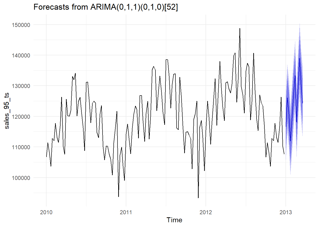
We’re fairly limited in what we can actually tweak when using
autoplot(), so instead we can convert the forecast object to a data
frame and use ggplot() like normal:
##          Point Forecast    Lo 80    Hi 80    Lo 95    Hi 95
## 2013.000       116571.1 109554.8 123587.5 105840.6 127301.7
## 2013.019       126102.0 119038.7 133165.2 115299.7 136904.3
## 2013.038       120871.5 113761.7 127981.4 109998.0 131745.1
## 2013.058       111934.8 104778.7 119091.0 100990.5 122879.2
## 2013.077       119470.2 112268.0 126672.3 108455.5 130484.9
## 2013.096       126904.7 119656.9 134152.5 115820.1 137989.3
## 2013.115       133382.4 126089.2 140675.6 122228.3 144536.5
## 2013.135       118094.6 110756.3 125433.0 106871.6 129317.7
## 2013.154       128769.9 121386.7 136153.1 117478.2 140061.6
## 2013.173       139022.7 131594.8 146450.5 127662.8 150382.5
## 2013.192       130502.1 123030.0 137974.3 119074.5 141929.8
## 2013.212       124236.7 116720.5 131752.9 112741.7 135731.7
## # A tibble: 324 × 7
## index key value lo.80 lo.95 hi.80 hi.95
## <dbl> <chr> <dbl> <dbl> <dbl> <dbl> <dbl>
## 1 2010 actual 106690. NA NA NA NA
## 2 2010. actual 111390. NA NA NA NA
## 3 2010. actual 107952. NA NA NA NA
## 4 2010. actual 103653. NA NA NA NA
## 5 2010. actual 112808. NA NA NA NA
## 6 2010. actual 112048. NA NA NA NA
## 7 2010. actual 117716. NA NA NA NA
## 8 2010. actual 113117. NA NA NA NA
## 9 2010. actual 111466. NA NA NA NA
## 10 2010. actual 116771. NA NA NA NA
## # … with 314 more rows## # A tibble: 324 × 8
## index key value lo.80 lo.95 hi.80 hi.95 actual_date
## <dbl> <chr> <dbl> <dbl> <dbl> <dbl> <dbl> <date>
## 1 2010 actual 106690. NA NA NA NA 1975-07-04
## 2 2010. actual 111390. NA NA NA NA 1975-07-04
## 3 2010. actual 107952. NA NA NA NA 1975-07-04
## 4 2010. actual 103653. NA NA NA NA 1975-07-04
## 5 2010. actual 112808. NA NA NA NA 1975-07-04
## 6 2010. actual 112048. NA NA NA NA 1975-07-04
## 7 2010. actual 117716. NA NA NA NA 1975-07-04
## 8 2010. actual 113117. NA NA NA NA 1975-07-04
## 9 2010. actual 111466. NA NA NA NA 1975-07-04
## 10 2010. actual 116771. NA NA NA NA 1975-07-04
## # … with 314 more rows
A Bit of Forecasting?
We are always interested in the future. We will do this in three ways:
- use Simple Exponential Smoothing
- use a package called
forecastto fit an ARIMA (Autoregressive Moving Average Integrated Model) model to the data and make predictions for weekly sales; - And do the same using a package called
Workflow using Orange
Workflow using Radiant
Workflow using R
Conclusion
References
1, Shampoo Dataset Brownlee: https://raw.githubusercontent.com/jbrownlee/Datasets/master/shampoo.csv
Arvind V.
My research interests are Complexity Science, Creativity and Innovation, Problem Solving with TRIZ, Literature, Indian Classical Music, and Computing with R.