👪 Populations, Samples, Statistics, and Inference
How much Data does a Man need?
What is a Population?
A population is a collection of individuals or observations we are
interested in. This is also commonly denoted as a study population. We
mathematically denote the population’s size using upper-case N.
A population parameter is some numerical summary about the population that is unknown but you wish you knew. For example, when this quantity is a mean like the average height of all Bangaloreans, the population parameter of interest is the population mean.
A census is an exhaustive enumeration or counting of all N individuals in the population. We do this in order to compute the population parameter’s value exactly. Of note is that as the number N of individuals in our population increases, conducting a census gets more expensive (in terms of time, energy, and money).
What is a Sample?
Sampling is the act of collecting a sample from the population, which we
generally do when we can’t perform a census. We mathematically denote
the sample size using lower case n, as opposed to upper case N which
denotes the population’s size. Typically the sample size n is much
smaller than the population size N. Thus sampling is a much cheaper
alternative than performing a census.
A sample statistic, also known as a point estimate, is a summary statistic like a mean or standard deviation that is computed from a sample.
Why do we sample?
Because we cannot conduct a census ( not always ) — and sometimes we won’t even know how big the population is — we take samples. And we still want to do useful work for/with the population, after estimating its parameters, an act of generalizing from sample to population. So the question is, can we estimate useful parameters of the population, using just samples? Can point estimates serve as useful guides to population parameters?
This act of generalizing from sample to population is at the heart of statistical inference.
NOTE: there is an alliterative mnemonic here: Samples have Statistics; Populations have Parameters.
Sampling
We will first execute some samples from a known dataset. We load up the NHANES dataset and inspect it.
data("NHANES")
mosaic::inspect(NHANES)
##
## categorical variables:
## name class levels n missing
## 1 SurveyYr factor 2 10000 0
## 2 Gender factor 2 10000 0
## 3 AgeDecade factor 8 9667 333
## 4 Race1 factor 5 10000 0
## 5 Race3 factor 6 5000 5000
## 6 Education factor 5 7221 2779
## 7 MaritalStatus factor 6 7231 2769
## 8 HHIncome factor 12 9189 811
## 9 HomeOwn factor 3 9937 63
## 10 Work factor 3 7771 2229
## 11 BMICatUnder20yrs factor 4 1274 8726
## 12 BMI_WHO factor 4 9603 397
## 13 Diabetes factor 2 9858 142
## 14 HealthGen factor 5 7539 2461
## 15 LittleInterest factor 3 6667 3333
## 16 Depressed factor 3 6673 3327
## 17 SleepTrouble factor 2 7772 2228
## 18 PhysActive factor 2 8326 1674
## 19 TVHrsDay factor 7 4859 5141
## 20 CompHrsDay factor 7 4863 5137
## 21 Alcohol12PlusYr factor 2 6580 3420
## 22 SmokeNow factor 2 3211 6789
## 23 Smoke100 factor 2 7235 2765
## 24 Smoke100n factor 2 7235 2765
## 25 Marijuana factor 2 4941 5059
## 26 RegularMarij factor 2 4941 5059
## 27 HardDrugs factor 2 5765 4235
## 28 SexEver factor 2 5767 4233
## 29 SameSex factor 2 5768 4232
## 30 SexOrientation factor 3 4842 5158
## 31 PregnantNow factor 3 1696 8304
## distribution
## 1 2009_10 (50%), 2011_12 (50%)
## 2 female (50.2%), male (49.8%)
## 3 40-49 (14.5%), 0-9 (14.4%) ...
## 4 White (63.7%), Black (12%) ...
## 5 White (62.7%), Black (11.8%) ...
## 6 Some College (31.4%) ...
## 7 Married (54.6%), NeverMarried (19.1%) ...
## 8 more 99999 (24.2%) ...
## 9 Own (64.7%), Rent (33.1%) ...
## 10 Working (59.4%), NotWorking (36.6%) ...
## 11 NormWeight (63.2%), Obese (17.3%) ...
## 12 18.5_to_24.9 (30.3%) ...
## 13 No (92.3%), Yes (7.7%)
## 14 Good (39.2%), Vgood (33.3%) ...
## 15 None (76.5%), Several (16.9%) ...
## 16 None (78.6%), Several (15.1%) ...
## 17 No (74.6%), Yes (25.4%)
## 18 Yes (55.8%), No (44.2%)
## 19 2_hr (26.2%), 1_hr (18.2%) ...
## 20 0_to_1_hr (29%), 0_hrs (22.1%) ...
## 21 Yes (79.2%), No (20.8%)
## 22 No (54.3%), Yes (45.7%)
## 23 No (55.6%), Yes (44.4%)
## 24 Non-Smoker (55.6%), Smoker (44.4%)
## 25 Yes (58.5%), No (41.5%)
## 26 No (72.4%), Yes (27.6%)
## 27 No (81.5%), Yes (18.5%)
## 28 Yes (96.1%), No (3.9%)
## 29 No (92.8%), Yes (7.2%)
## 30 Heterosexual (95.8%), Bisexual (2.5%) ...
## 31 No (92.7%), Yes (4.2%) ...
##
## quantitative variables:
## name class min Q1 median Q3 max
## 1 ID integer 51624.00 56904.500 62159.500 67039.000 71915.000
## 2 Age integer 0.00 17.000 36.000 54.000 80.000
## 3 AgeMonths integer 0.00 199.000 418.000 624.000 959.000
## 4 HHIncomeMid integer 2500.00 30000.000 50000.000 87500.000 100000.000
## 5 Poverty numeric 0.00 1.240 2.700 4.710 5.000
## 6 HomeRooms integer 1.00 5.000 6.000 8.000 13.000
## 7 Weight numeric 2.80 56.100 72.700 88.900 230.700
## 8 Length numeric 47.10 75.700 87.000 96.100 112.200
## 9 HeadCirc numeric 34.20 39.575 41.450 42.925 45.400
## 10 Height numeric 83.60 156.800 166.000 174.500 200.400
## 11 BMI numeric 12.88 21.580 25.980 30.890 81.250
## 12 Pulse integer 40.00 64.000 72.000 82.000 136.000
## 13 BPSysAve integer 76.00 106.000 116.000 127.000 226.000
## 14 BPDiaAve integer 0.00 61.000 69.000 76.000 116.000
## 15 BPSys1 integer 72.00 106.000 116.000 128.000 232.000
## 16 BPDia1 integer 0.00 62.000 70.000 76.000 118.000
## 17 BPSys2 integer 76.00 106.000 116.000 128.000 226.000
## 18 BPDia2 integer 0.00 60.000 68.000 76.000 118.000
## 19 BPSys3 integer 76.00 106.000 116.000 126.000 226.000
## 20 BPDia3 integer 0.00 60.000 68.000 76.000 116.000
## 21 Testosterone numeric 0.25 17.700 43.820 362.410 1795.600
## 22 DirectChol numeric 0.39 1.090 1.290 1.580 4.030
## 23 TotChol numeric 1.53 4.110 4.780 5.530 13.650
## 24 UrineVol1 integer 0.00 50.000 94.000 164.000 510.000
## 25 UrineFlow1 numeric 0.00 0.403 0.699 1.221 17.167
## 26 UrineVol2 integer 0.00 52.000 95.000 171.750 409.000
## 27 UrineFlow2 numeric 0.00 0.475 0.760 1.513 13.692
## 28 DiabetesAge integer 1.00 40.000 50.000 58.000 80.000
## 29 DaysPhysHlthBad integer 0.00 0.000 0.000 3.000 30.000
## 30 DaysMentHlthBad integer 0.00 0.000 0.000 4.000 30.000
## 31 nPregnancies integer 1.00 2.000 3.000 4.000 32.000
## 32 nBabies integer 0.00 2.000 2.000 3.000 12.000
## 33 Age1stBaby integer 14.00 19.000 22.000 26.000 39.000
## 34 SleepHrsNight integer 2.00 6.000 7.000 8.000 12.000
## 35 PhysActiveDays integer 1.00 2.000 3.000 5.000 7.000
## 36 TVHrsDayChild integer 0.00 1.000 2.000 3.000 6.000
## 37 CompHrsDayChild integer 0.00 0.000 1.000 6.000 6.000
## 38 AlcoholDay integer 1.00 1.000 2.000 3.000 82.000
## 39 AlcoholYear integer 0.00 3.000 24.000 104.000 364.000
## 40 SmokeAge integer 6.00 15.000 17.000 19.000 72.000
## 41 AgeFirstMarij integer 1.00 15.000 16.000 19.000 48.000
## 42 AgeRegMarij integer 5.00 15.000 17.000 19.000 52.000
## 43 SexAge integer 9.00 15.000 17.000 19.000 50.000
## 44 SexNumPartnLife integer 0.00 2.000 5.000 12.000 2000.000
## 45 SexNumPartYear integer 0.00 1.000 1.000 1.000 69.000
## mean sd n missing
## 1 6.194464e+04 5.871167e+03 10000 0
## 2 3.674210e+01 2.239757e+01 10000 0
## 3 4.201239e+02 2.590431e+02 4962 5038
## 4 5.720617e+04 3.302028e+04 9189 811
## 5 2.801844e+00 1.677909e+00 9274 726
## 6 6.248918e+00 2.277538e+00 9931 69
## 7 7.098180e+01 2.912536e+01 9922 78
## 8 8.501602e+01 1.370503e+01 543 9457
## 9 4.118068e+01 2.311483e+00 88 9912
## 10 1.618778e+02 2.018657e+01 9647 353
## 11 2.666014e+01 7.376579e+00 9634 366
## 12 7.355973e+01 1.215542e+01 8563 1437
## 13 1.181550e+02 1.724817e+01 8551 1449
## 14 6.748006e+01 1.435480e+01 8551 1449
## 15 1.190902e+02 1.749636e+01 8237 1763
## 16 6.827826e+01 1.378078e+01 8237 1763
## 17 1.184758e+02 1.749133e+01 8353 1647
## 18 6.766455e+01 1.441978e+01 8353 1647
## 19 1.179292e+02 1.717719e+01 8365 1635
## 20 6.729874e+01 1.495839e+01 8365 1635
## 21 1.978980e+02 2.265045e+02 4126 5874
## 22 1.364865e+00 3.992581e-01 8474 1526
## 23 4.879220e+00 1.075583e+00 8474 1526
## 24 1.185161e+02 9.033648e+01 9013 987
## 25 9.792946e-01 9.495143e-01 8397 1603
## 26 1.196759e+02 9.016005e+01 1478 8522
## 27 1.149372e+00 1.072948e+00 1476 8524
## 28 4.842289e+01 1.568050e+01 629 9371
## 29 3.334838e+00 7.400700e+00 7532 2468
## 30 4.126493e+00 7.832971e+00 7534 2466
## 31 3.026882e+00 1.795341e+00 2604 7396
## 32 2.456954e+00 1.315227e+00 2416 7584
## 33 2.264968e+01 4.772509e+00 1884 8116
## 34 6.927531e+00 1.346729e+00 7755 2245
## 35 3.743513e+00 1.836358e+00 4663 5337
## 36 1.938744e+00 1.434431e+00 653 9347
## 37 2.197550e+00 2.516667e+00 653 9347
## 38 2.914123e+00 3.182672e+00 4914 5086
## 39 7.510165e+01 1.030337e+02 5922 4078
## 40 1.782662e+01 5.326660e+00 3080 6920
## 41 1.702283e+01 3.895010e+00 2891 7109
## 42 1.769107e+01 4.806103e+00 1366 8634
## 43 1.742870e+01 3.716551e+00 5540 4460
## 44 1.508507e+01 5.784643e+01 5725 4275
## 45 1.342330e+00 2.782688e+00 4928 5072Let us create a NHANES dataset without duplicated IDs and only adults:
NHANES <-
  NHANES %>%
  distinct(ID, .keep_all = TRUE)

#create a dataset of only adults
NHANES_adult <-
  NHANES %>%
  filter(Age >= 18) %>%
  drop_na(Height)

glimpse(NHANES_adult)
## Rows: 4,790
## Columns: 76
## $ ID <int> 51624, 51630, 51647, 51654, 51656, 51657, 51666, 5166…
## $ SurveyYr <fct> 2009_10, 2009_10, 2009_10, 2009_10, 2009_10, 2009_10,…
## $ Gender <fct> male, female, female, male, male, male, female, male,…
## $ Age <int> 34, 49, 45, 66, 58, 54, 58, 50, 33, 60, 56, 57, 54, 3…
## $ AgeDecade <fct> 30-39, 40-49, 40-49, 60-69, 50-59, 50-59, 50-5…
## $ AgeMonths <int> 409, 596, 541, 795, 707, 654, 700, 603, 404, 721, 677…
## $ Race1 <fct> White, White, White, White, White, White, Mexican, Wh…
## $ Race3 <fct> NA, NA, NA, NA, NA, NA, NA, NA, NA, NA, NA, NA, NA, N…
## $ Education <fct> High School, Some College, College Grad, Some College…
## $ MaritalStatus <fct> Married, LivePartner, Married, Married, Divorced, Mar…
## $ HHIncome <fct> 25000-34999, 35000-44999, 75000-99999, 25000-34999, m…
## $ HHIncomeMid <int> 30000, 40000, 87500, 30000, 100000, 70000, 87500, 175…
## $ Poverty <dbl> 1.36, 1.91, 5.00, 2.20, 5.00, 2.20, 2.03, 1.24, 1.27,…
## $ HomeRooms <int> 6, 5, 6, 5, 10, 6, 10, 4, 11, 5, 10, 9, 3, 6, 6, 10, …
## $ HomeOwn <fct> Own, Rent, Own, Own, Rent, Rent, Rent, Rent, Own, Own…
## $ Work <fct> NotWorking, NotWorking, Working, NotWorking, Working,…
## $ Weight <dbl> 87.4, 86.7, 75.7, 68.0, 78.4, 74.7, 57.5, 84.1, 93.8,…
## $ Length <dbl> NA, NA, NA, NA, NA, NA, NA, NA, NA, NA, NA, NA, NA, N…
## $ HeadCirc <dbl> NA, NA, NA, NA, NA, NA, NA, NA, NA, NA, NA, NA, NA, N…
## $ Height <dbl> 164.7, 168.4, 166.7, 169.5, 181.9, 169.4, 148.1, 177.…
## $ BMI <dbl> 32.22, 30.57, 27.24, 23.67, 23.69, 26.03, 26.22, 26.6…
## $ BMICatUnder20yrs <fct> NA, NA, NA, NA, NA, NA, NA, NA, NA, NA, NA, NA, NA, N…
## $ BMI_WHO <fct> 30.0_plus, 30.0_plus, 25.0_to_29.9, 18.5_to_24.9, 18.…
## $ Pulse <int> 70, 86, 62, 60, 62, 76, 94, 74, 96, 84, 64, 70, 64, 6…
## $ BPSysAve <int> 113, 112, 118, 111, 104, 134, 127, 142, 128, 152, 95,…
## $ BPDiaAve <int> 85, 75, 64, 63, 74, 85, 83, 68, 74, 100, 69, 89, 41, …
## $ BPSys1 <int> 114, 118, 106, 124, 108, 136, NA, 138, 126, 154, 94, …
## $ BPDia1 <int> 88, 82, 62, 64, 76, 86, NA, 66, 80, 98, 74, 82, 48, 8…
## $ BPSys2 <int> 114, 108, 118, 108, 104, 132, 134, 142, 128, 150, 94,…
## $ BPDia2 <int> 88, 74, 68, 62, 72, 88, 82, 74, 74, 98, 70, 88, 42, 8…
## $ BPSys3 <int> 112, 116, 118, 114, 104, 136, 120, 142, NA, 154, 96, …
## $ BPDia3 <int> 82, 76, 60, 64, 76, 82, 84, 62, NA, 102, 68, 90, 40, …
## $ Testosterone <dbl> NA, NA, NA, NA, NA, NA, NA, NA, NA, NA, NA, NA, NA, N…
## $ DirectChol <dbl> 1.29, 1.16, 2.12, 0.67, 0.96, 1.16, 1.14, 1.06, 0.91,…
## $ TotChol <dbl> 3.49, 6.70, 5.82, 4.99, 4.24, 6.41, 4.78, 5.22, 5.59,…
## $ UrineVol1 <int> 352, 77, 106, 113, 163, 215, 29, 64, 155, 238, 26, 13…
## $ UrineFlow1 <dbl> NA, 0.094, 1.116, 0.489, NA, 0.903, 0.299, 0.190, 0.5…
## $ UrineVol2 <int> NA, NA, NA, NA, NA, NA, NA, NA, NA, NA, 86, NA, NA, N…
## $ UrineFlow2 <dbl> NA, NA, NA, NA, NA, NA, NA, NA, NA, NA, 0.43, NA, NA,…
## $ Diabetes <fct> No, No, No, No, No, No, No, No, No, No, No, No, No, N…
## $ DiabetesAge <int> NA, NA, NA, NA, NA, NA, NA, NA, NA, NA, NA, NA, NA, N…
## $ HealthGen <fct> Good, Good, Vgood, Vgood, Vgood, Fair, NA, Good, Fair…
## $ DaysPhysHlthBad <int> 0, 0, 0, 10, 0, 4, NA, 0, 3, 7, 3, 0, 0, 3, 0, 2, 0, …
## $ DaysMentHlthBad <int> 15, 10, 3, 0, 0, 0, NA, 0, 7, 0, 0, 0, 0, 4, 0, 30, 0…
## $ LittleInterest <fct> Most, Several, None, None, None, None, NA, None, Seve…
## $ Depressed <fct> Several, Several, None, None, None, None, NA, None, N…
## $ nPregnancies <int> NA, 2, 1, NA, NA, NA, NA, NA, NA, NA, 4, 2, NA, NA, N…
## $ nBabies <int> NA, 2, NA, NA, NA, NA, NA, NA, NA, NA, 3, 2, NA, NA, …
## $ Age1stBaby <int> NA, 27, NA, NA, NA, NA, NA, NA, NA, NA, 26, 32, NA, N…
## $ SleepHrsNight <int> 4, 8, 8, 7, 5, 4, 5, 7, 6, 6, 7, 8, 6, 5, 6, 4, 5, 7,…
## $ SleepTrouble <fct> Yes, Yes, No, No, No, Yes, No, No, No, Yes, No, No, Y…
## $ PhysActive <fct> No, No, Yes, Yes, Yes, Yes, Yes, Yes, No, No, Yes, Ye…
## $ PhysActiveDays <int> NA, NA, 5, 7, 5, 1, 2, 7, NA, NA, 7, 3, 3, NA, 2, NA,…
## $ TVHrsDay <fct> NA, NA, NA, NA, NA, NA, NA, NA, NA, NA, NA, NA, NA, N…
## $ CompHrsDay <fct> NA, NA, NA, NA, NA, NA, NA, NA, NA, NA, NA, NA, NA, N…
## $ TVHrsDayChild <int> NA, NA, NA, NA, NA, NA, NA, NA, NA, NA, NA, NA, NA, N…
## $ CompHrsDayChild <int> NA, NA, NA, NA, NA, NA, NA, NA, NA, NA, NA, NA, NA, N…
## $ Alcohol12PlusYr <fct> Yes, Yes, Yes, Yes, Yes, Yes, NA, No, Yes, Yes, Yes, …
## $ AlcoholDay <int> NA, 2, 3, 1, 2, 6, NA, NA, 3, 6, 1, 1, 2, NA, 12, NA,…
## $ AlcoholYear <int> 0, 20, 52, 100, 104, 364, NA, 0, 104, 36, 12, 312, 15…
## $ SmokeNow <fct> No, Yes, NA, No, NA, NA, Yes, NA, No, No, NA, No, NA,…
## $ Smoke100 <fct> Yes, Yes, No, Yes, No, No, Yes, No, Yes, Yes, No, Yes…
## $ Smoke100n <fct> Smoker, Smoker, Non-Smoker, Smoker, Non-Smoker, Non-S…
## $ SmokeAge <int> 18, 38, NA, 13, NA, NA, 17, NA, NA, 16, NA, 18, NA, N…
## $ Marijuana <fct> Yes, Yes, Yes, NA, Yes, Yes, NA, No, No, NA, No, Yes,…
## $ AgeFirstMarij <int> 17, 18, 13, NA, 19, 15, NA, NA, NA, NA, NA, 18, NA, N…
## $ RegularMarij <fct> No, No, No, NA, Yes, Yes, NA, No, No, NA, No, No, No,…
## $ AgeRegMarij <int> NA, NA, NA, NA, 20, 15, NA, NA, NA, NA, NA, NA, NA, N…
## $ HardDrugs <fct> Yes, Yes, No, No, Yes, Yes, NA, No, No, No, No, No, N…
## $ SexEver <fct> Yes, Yes, Yes, Yes, Yes, Yes, NA, Yes, Yes, Yes, Yes,…
## $ SexAge <int> 16, 12, 13, 17, 22, 12, NA, NA, 27, 20, 20, 18, 14, 2…
## $ SexNumPartnLife <int> 8, 10, 20, 15, 7, 100, NA, 9, 1, 1, 2, 5, 20, 1, 20, …
## $ SexNumPartYear <int> 1, 1, 0, NA, 1, 1, NA, 1, 1, NA, 1, 1, 2, 1, 3, 1, NA…
## $ SameSex <fct> No, Yes, Yes, No, No, No, NA, No, No, No, No, No, No,…
## $ SexOrientation <fct> Heterosexual, Heterosexual, Bisexual, NA, Heterosexua…
## $ PregnantNow <fct> NA, NA, NA, NA, NA, NA, NA, NA, NA, NA, NA, NA, NA, N…For now, we will treat this dataset as our Population. So each
variable in the dataset is a population for that particular
quantity/category, with appropriate population parameters such as
means, sd-s, and proportions. Let us calculate the population
parameters for the Height data:
pop_mean_height <- mean(~ Height, data = NHANES_adult)
pop_sd_height <- sd(~ Height, data = NHANES_adult)

pop_mean_height
## [1] 168.3497pop_sd_height## [1] 10.15705One Sample
Now, we will sample ONCE from the NHANES Height variable. Let us
take a sample of sample size 50. We will compare sample statistics
with population parameters on the basis of this ONE sample of 50:
sample_height <- sample(NHANES_adult, size = 50) %>% select(Height)
sample_height
## # A tibble: 50 × 1
## Height
## <dbl>
## 1 172
## 2 159.
## 3 171
## 4 159.
## 5 156.
## 6 170.
## 7 148.
## 8 159.
## 9 168.
## 10 159.
## # … with 40 more rowssample_mean_height <- mean(~ Height, data = sample_height)
sample_mean_height## [1] 165.866# Plotting the histogram of this sample
sample_height %>% gf_histogram(~ Height) %>%
gf_vline(xintercept = sample_mean_height, color = "red") %>%
gf_vline(xintercept = pop_mean_height, colour = "blue") %>%
gf_text(1 ~ (pop_mean_height + 5), label = "Population Mean Height", color = "blue") %>%
gf_text(2 ~ (sample_mean_height-5), label = "Sample Mean Height", color = "red")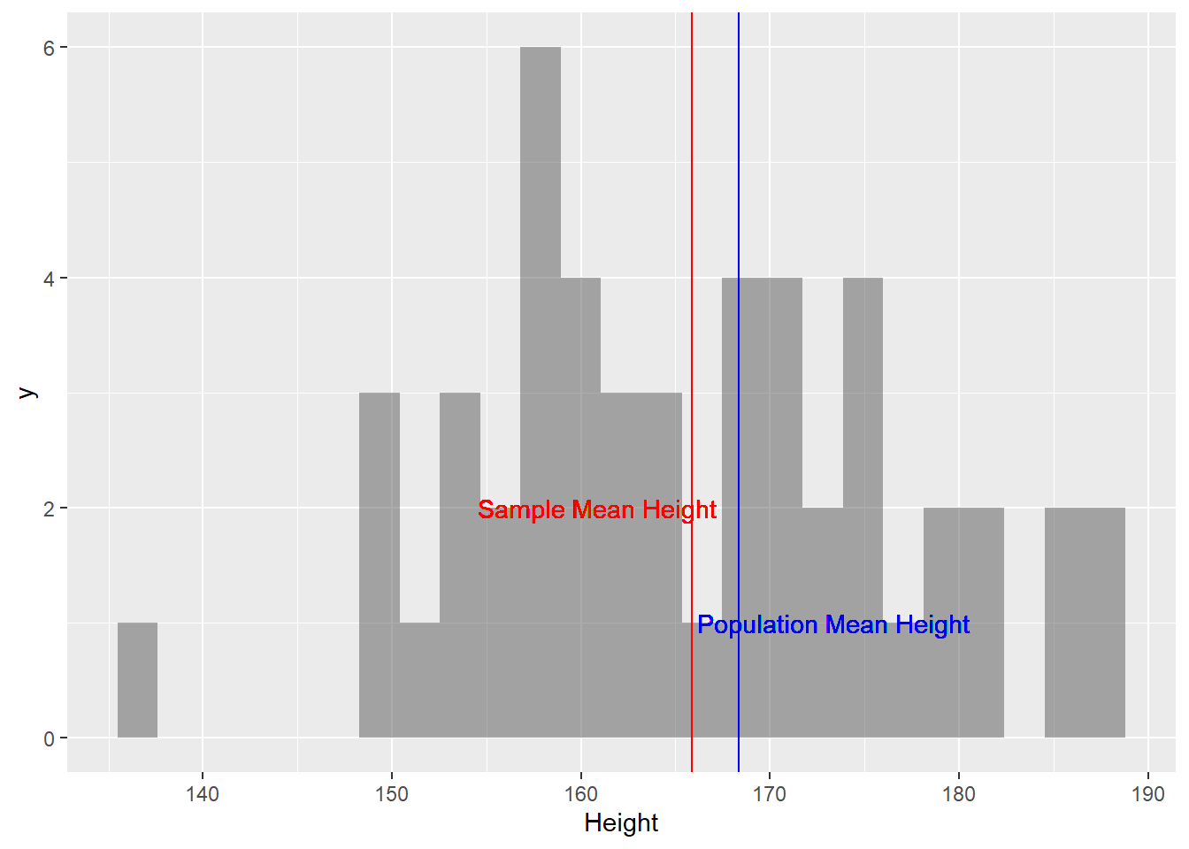
Figure 1: Single-Sample Mean and Population Mean
500 Samples
OK, so the sample_mean_height is not too far from the
pop_mean_height. Is this always true? Let us check: we will create 500
samples each of size 50. And calculate their mean as the sample
statistic, giving us a dataframe containing 5000 sample means. We
will then compare if these 500 means are close to the pop_mean_height:
sample_height_500 <- do(500) * {
  sample(NHANES_adult, size = 50) %>%
    select(Height) %>%
    summarise(
      sample_mean_500 = mean(Height),
      sample_min_500 = min(Height),
      sample_max_500 = max(Height))
}

head(sample_height_500)
## # A tibble: 6 × 5
## sample_mean_500 sample_min_500 sample_max_500 .row .index
## <dbl> <dbl> <dbl> <int> <dbl>
## 1 167. 144. 189. 1 1
## 2 167. 144. 191. 1 2
## 3 167. 147. 192. 1 3
## 4 170. 147. 192. 1 4
## 5 169 149. 191. 1 5
## 6 166. 143. 188. 1 6dim(sample_height_500)## [1] 500 5sample_height_500 %>%
gf_point(.index ~ sample_mean_500, color = "red") %>%
gf_segment(
.index + .index ~ sample_min_500 + sample_max_500,
color = "red",
size = 0.3,
alpha = 0.3,
ylab = "Sample Index (1-500)",
xlab = "Sample Means"
) %>%
gf_vline(xintercept = ~ pop_mean_height, color = "blue") %>%
gf_label(-15 ~ pop_mean_height, label = "Population Mean", color = "blue")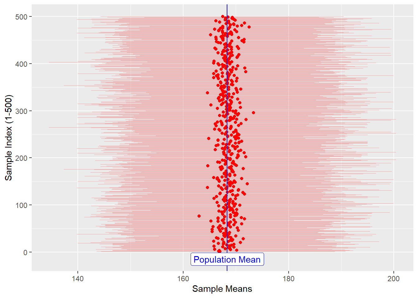
Figure 2: Multiple Sample-Means and Population Mean
The sample_means (red dots), are themselves random because the samples
are random, of course. It appears that they are generally in the
vicinity of the pop_mean (blue line).
Distribution of Sample-Means
Since the sample-means are themselves random variables, let’s plot the distribution of these 5000 sample-means themselves, called a a distribution of sample-means.
NOTE: this a distribution of sample-means will itself have a mean and standard deviation. Do not get confused ;-D
We will also plot the position of the population mean pop_mean_height
parameter, the means of the Height variable.
sample_height_500 %>% gf_dhistogram(~ sample_mean_500) %>%
  gf_vline(xintercept = pop_mean_height, color = "blue") %>%
   gf_label(0.01 ~ pop_mean_height, label = "Population Mean", color = "blue")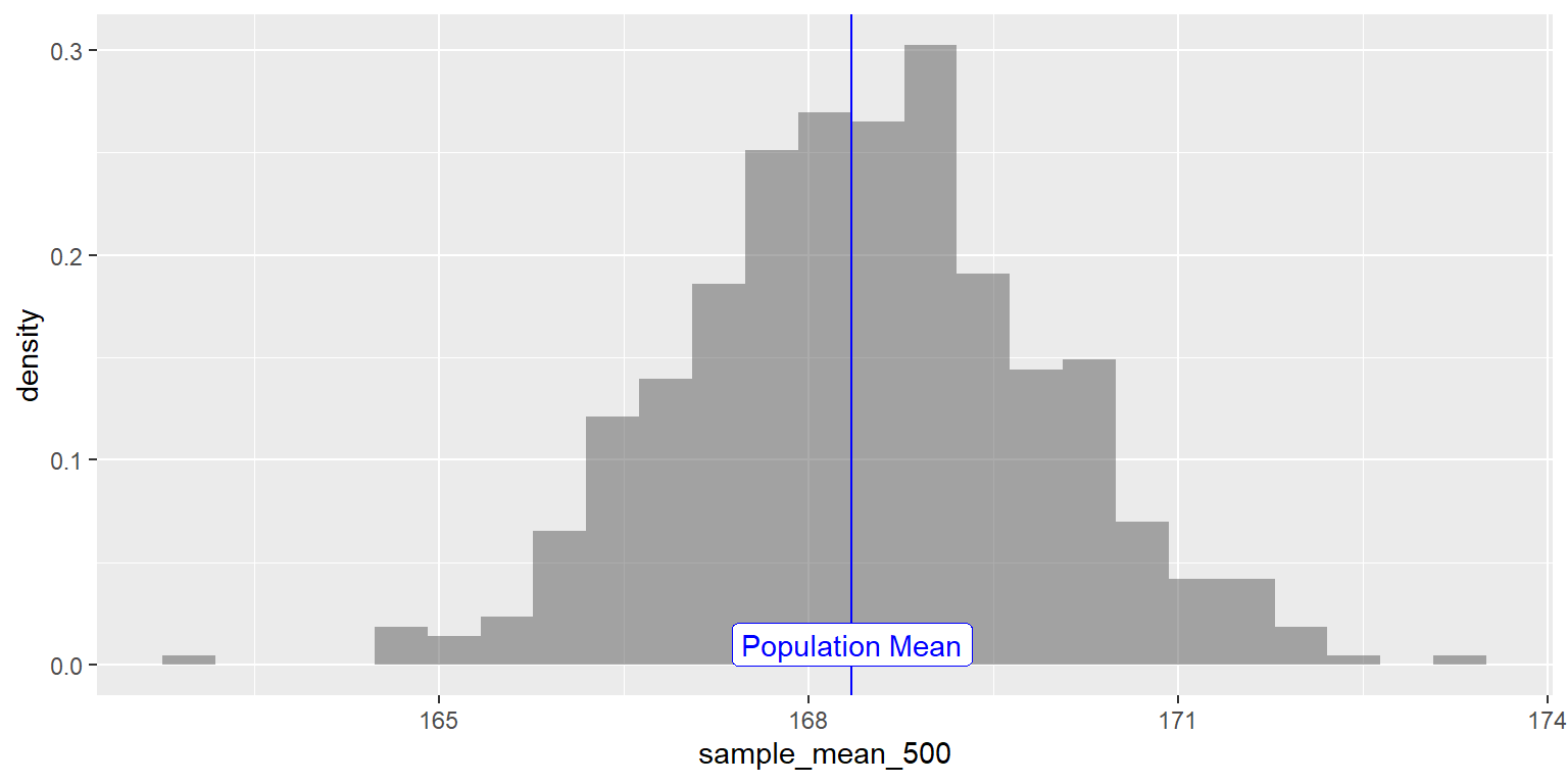
Figure 3: Sampling Mean Distribution
How does this distribution of sample-means compare with that of the overall distribution of the population heights?
sample_height_500 %>% gf_dhistogram(~ sample_mean_500,bins = 50,fill = "red") %>%
  gf_vline(xintercept = pop_mean_height, color = "blue") %>%
   gf_label(0.01 ~ pop_mean_height, label = "Population Mean", color = "blue") %>%

  ## Add the population histogram
  gf_histogram(~ Height, data = NHANES_adult, alpha = 0.2, fill = "blue", bins = 50) %>%
  gf_label(0.025 ~ (pop_mean_height + 20), label = "Population Distribution of Height", color = "blue") %>%
    gf_label(0.25 ~ (pop_mean_height + 17), label = "Distribution of 500 Height Sample Means", color = "red")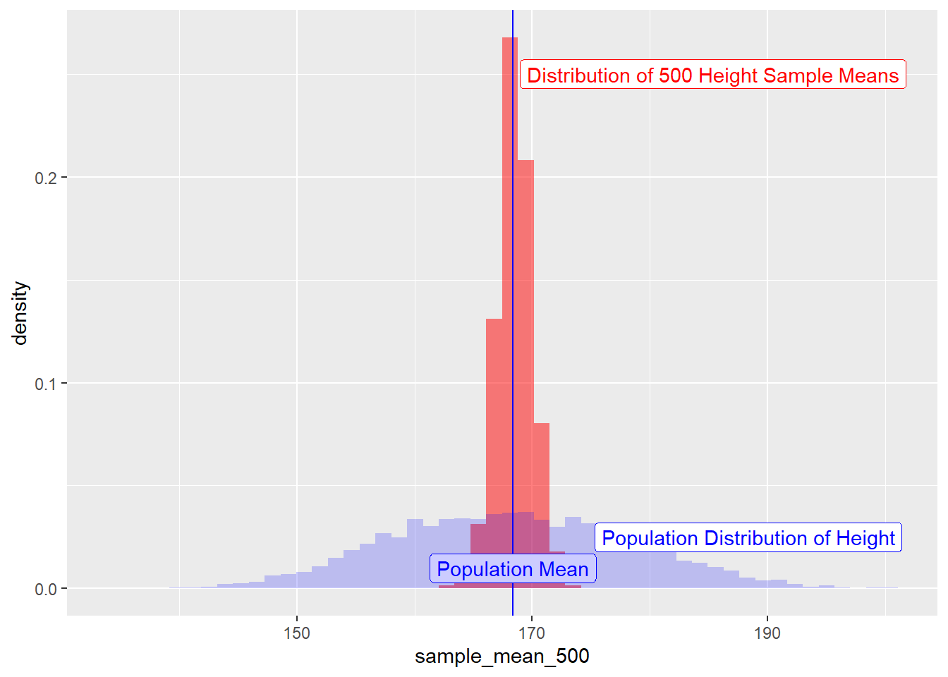
Figure 4: Sampling Means and Population Distributions
Central limit theorem
We see in the Figure above that
- the distribution of sample-means is centered around mean =
pop_mean. - That the standard deviation of the distribution of sample means is less than that of the original population. But exactly what is it?
- And what is the kind of distribution?
One more experiment.
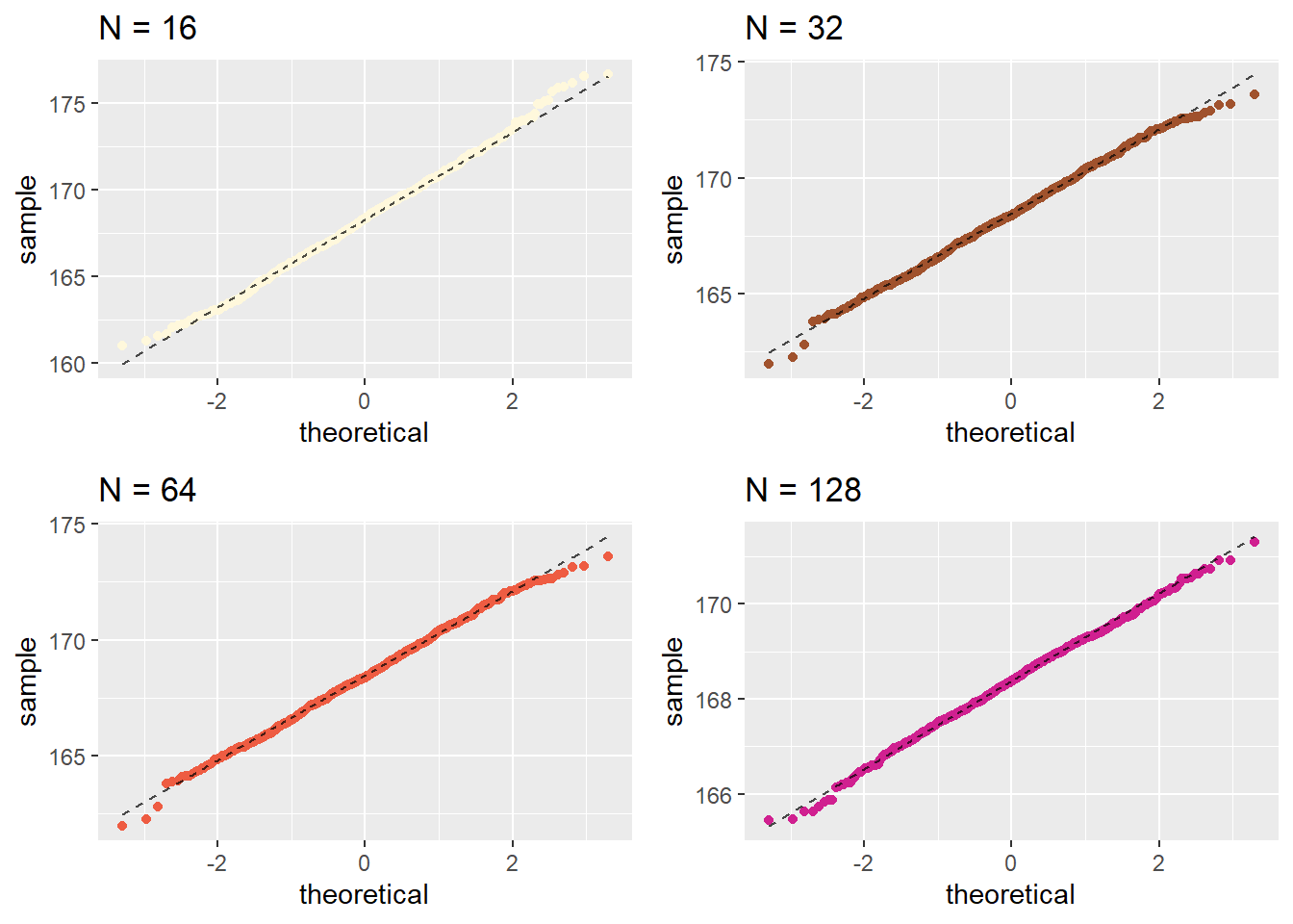
Now let’s repeatedly sample Height and compute the sample mean, and
look at the resulting histograms and Q-Q plots. ( Q-Q plots check
whether a certain distribution is close to being normal or not.)
We will use sample sizes of c(16, 32, 64, 128) and generate 1000
samples each time, take the means and plot these 1000 means:
set.seed(12345)


samples_height_16 <- do(1000) * mean(resample(NHANES_adult$Height, size = 16))
samples_height_32 <- do(1000) * mean(resample(NHANES_adult$Height, size = 32))
samples_height_64 <- do(1000) * mean(resample(NHANES_adult$Height, size = 64))
samples_height_128 <- do(1000) * mean(resample(NHANES_adult$Height, size = 128))

# Quick Check
head(samples_height_16)
## mean
## 1 168.0500
## 2 166.1000
## 3 165.5375
## 4 167.5625
## 5 165.2375
## 6 169.0250### do(1000,) * mean(resample(NHANES_adult$Height, size = 16)) produces a data frame with a variable named mean.
###Now let’s create separate Q-Q plots for the different sample sizes.
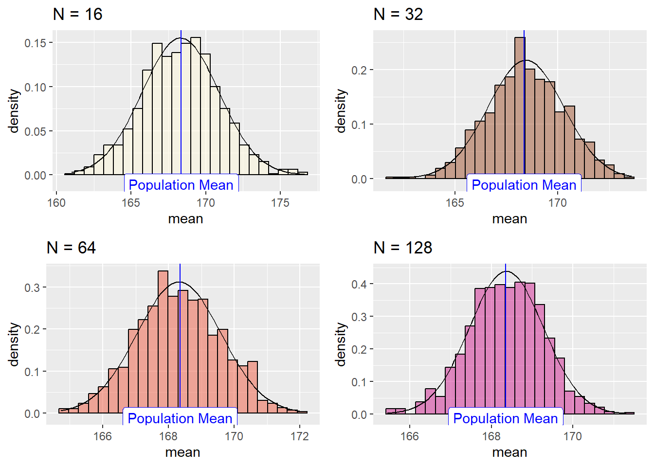
Let us plot their individual histograms to compare them:
And if we overlay the histograms:
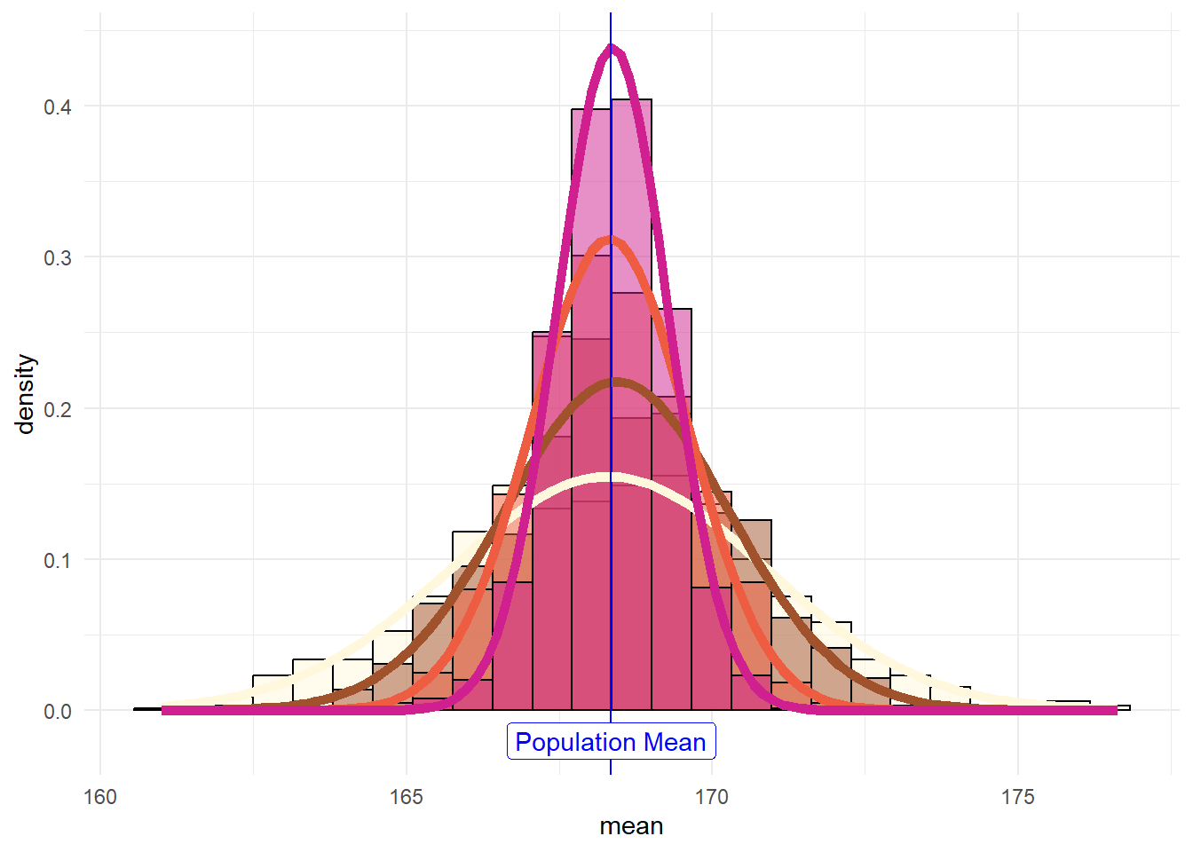
This shows that the results become more normally distributed (i.e. following the straight line) as the samples get larger. Hence we learn that:
- the sample-means are normally distributed around the population mean. This is because when we sample from the population, many values will be close to the population mean, and values far away from the mean will be increasingly scarce.
mean(~ mean, data  = samples_height_16)
mean(~ mean, data  = samples_height_32)
mean(~ mean, data  = samples_height_64)
mean(~ mean, data  = samples_height_128)
pop_mean_height
## [1] 168.306
## [1] 168.4349
## [1] 168.3184
## [1] 168.366
## [1] 168.3497the sample-means become “more normally distributed” with sample length, as shown by the (small but definite) improvements in the Q-Q plots with sample-size.
the sample-mean distributions narrow with sample length.
This is regardless of the distribution of the population itself. (
The Height variable seems to be normally distributed at population
level. We will try other non-normal population variables as an
exercise). This is the Central Limit Theorem (CLT).
As we saw in the figure above, the standard deviations of the sample-mean distributions reduce with sample size. In fact their SDs are defined by:
sd = pop_sd/sqrt(sample_size) where sample-size here is one of
c(16,32,64,128)
sd(~ mean, data  = samples_height_16)
sd(~ mean, data  = samples_height_32)
sd(~ mean, data  = samples_height_64)
sd(~ mean, data  = samples_height_128)
## [1] 2.578355
## [1] 1.834979
## [1] 1.280014
## [1] 0.9096318The standard deviation of the sample-mean distribution is called the Standard Error. This statistic derived from the sample, will help us infer our population parameters with a precise estimate of the uncertainty involved.
\[ Standard\ Error\ {\pmb {se} = \frac{population\ sd}{\sqrt[]{sample\ size}}}\\\\ \\ \pmb {se} = \frac{\sigma}{\sqrt[]{n}}\\ \]
In our sampling experiments, the Standard Errors evaluate to:
pop_sd_height <- sd(~ Height, data = NHANES_adult)

pop_sd_height/sqrt(16)
pop_sd_height/sqrt(32)
pop_sd_height/sqrt(64)
pop_sd_height/sqrt(128)
## [1] 2.539262
## [1] 1.795529
## [1] 1.269631
## [1] 0.8977646As seen, these are identical to the Standard Deviations of the individual sample-mean distributions.
Confidence intervals
When we work with samples, we want to be able to speak with a certain degree of confidence about the population mean, based on the evaluation of one sample mean,not a whole large number of them. Give that sample-means are normally distributed around the population means, we can say that \(68%\) of all possible sample-mean lie within $ +/- 1 SE $ of the population mean; and further that \(95%\) of of all possible sample-mean lie within $ +/- 1.5* SE $ of the population mean.
These two intervals [sample-mean +/- SE] and [sample-mean +/- 1.5SE] are called the confidence intervals for the population mean, at levels 68% and 95% respectively.
Thus if we want to estimate a population mean:\
- we take one sample of size \(n\) from the population
- we calculate the sample-mean - we calculate the sample-sd
- We calculate the Standard Error as \(\frac{sample-sd}{\sqrt[]{n}}\)
- We calculate 95% confidence intervals for the population mean based on
the formula above.
Now that we have our basics ready, it is time to play with a dataset in the different tools at our disposal.
References
Diez, David M & Barr, Christopher D & Çetinkaya-Rundel, Mine, OpenIntro Statistics. https://www.openintro.org/book/os/
Stats Test Wizard. https://www.socscistatistics.com/tests/what_stats_test_wizard.aspx
Diez, David M & Barr, Christopher D & Çetinkaya-Rundel, Mine: OpenIntro Statistics. Available online https://www.openintro.org/book/os/
Måns Thulin, Modern Statistics with R: From wrangling and exploring data to inference and predictive modelling http://www.modernstatisticswithr.com/
Jonas Kristoffer Lindeløv, Common statistical tests are linear models (or: how to teach stats) https://lindeloev.github.io/tests-as-linear/
CheatSheet https://lindeloev.github.io/tests-as-linear/linear_tests_cheat_sheet.pdf
Common statistical tests are linear models: a work through by Steve Doogue https://steverxd.github.io/Stat_tests/
Jeffrey Walker “Elements of Statistical Modeling for Experimental Biology”. https://www.middleprofessor.com/files/applied-biostatistics_bookdown/_book/
Arvind V.
My research interests are Complexity Science, Creativity and Innovation, Problem Solving with TRIZ, Literature, Indian Classical Music, and Computing with R.