 Photo by rawpixel on Unsplash
What Graphs will we see today?
There are a good few charts available to depict things that constitute other bigger things. We will discuss a few of these: Pie, Fan, and Donuts; Waffle and Parliament charts; Trees, Dendrograms, and Circle Packings.
We will begin with Pie Charts, Fan Plots, and Donuts. We will then try to depict here the interesting ones such as the dendrogram, the parliament plot, the waffle plot, and the circle packing chart.
Pies and Fans
So let us start with “eating humble pie”: discussing a Pie chart first.
A pie chart is a circle divided into sectors that each represent a
proportion of the whole. It is often used to show percentage, where the
sum of the sectors equals 100%.
The problem is that humans are pretty bad at reading angles. This
ubiquitous chart is much vilified in the industry and bar charts that
we have seen earlier, are viewed as better options. However do read this
spirited defense of pie charts here.
https://speakingppt.com/why-tufte-is-flat-out-wrong-about-pie-charts/
On the other hand, pie charts are ubiquitous in business circles, and
are very much accepted ! So there is an attractive, and similar-looking
alternative, called a fan chart which we will explore here.
(Base) R has a simple pie command that does the job.
pie.sales <- c(0.12, 0.3, 0.26, 0.16, 0.04, 0.12)
labels <- c("Blueberry", "Cherry",
    "Apple", "Boston Cream", "Other", "Vanilla Cream")
pie(x = pie.sales, labels = labels,col =  grDevices::hcl.colors(palette= "Plasma", n = 6)) # default colours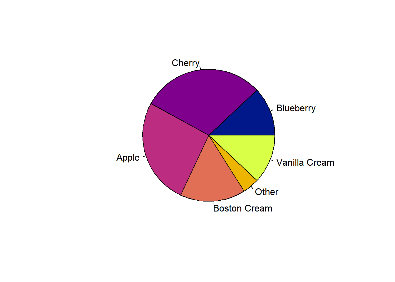
The fan plot displays numerical values as arcs of overlapping sectors. This allows for more effective comparison:
plotrix::fan.plot(x = pie.sales, labels = labels,
                  col = grDevices::hcl.colors(palette= "Plasma", n = 6),
                  shrink = 0.03, # How much to shrink each successive sector
                  label.radius = 1.15,
                  main = "Fan Plot of Ice Cream Flavours",
                  ticks = 360,
                  max.span = pi)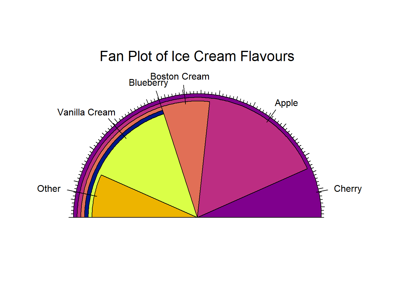
The donut chart suffers from the same defects as the pie, so should be
used with discretion. The donut chart is essentially a geom_rect
from ggplot, plotted on a polar coordinate set of of axes:
# Data
df <- data.frame(group = LETTERS[1:3],
                 value = c(25, 20, 35))

df <-
  df %>% dplyr::mutate(
    fraction = value / sum(value), # percentages
    ymax = cumsum(fraction), # cumulative percentages
    ymin = lag(ymax, 1, default = 0),
    # bottom edge of each
    label = paste0(group, "\n value: ", value),
    labelPosition = (ymax + ymin) / 2 # labels midway on arcs
  )

df
## group value fraction ymax ymin label labelPosition
## 1 A 25 0.3125 0.3125 0.0000 A\n value: 25 0.15625
## 2 B 20 0.2500 0.5625 0.3125 B\n value: 20 0.43750
## 3 C 35 0.4375 1.0000 0.5625 C\n value: 35 0.78125ggplot(df) +
# `geom_rect()` requires aesthetics: xmin, xmax, ymin, and ymax
geom_rect(aes(xmin = 2, xmax = 4, ymin = ymin, ymax = ymax, fill = group),colour = "black") +
geom_label( x=3.5, aes(y=labelPosition, label= label), size=4) +
coord_polar(theta = "y",direction = 1) + # Upto here will give us a pie chart
# When switching to polar coords:
# x maps to r
# y maps to theta
# so we create a "hole" in the radius, in in
xlim(c(0,4)) + # try to play with the "0"
theme_void() +
theme(legend.position = "none")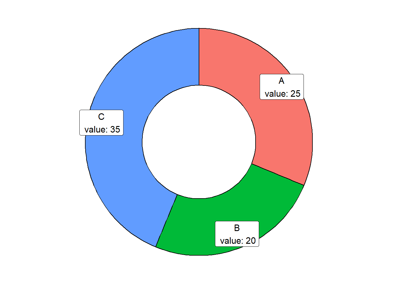
Parliament and Waffle Charts
Waffle charts are often called “square pie charts” !
# install.packages("waffle", repos = "https://cinc.rud.is")
library(waffle)

# Data
df <- data.frame(group = LETTERS[1:3],
                 value = c(25, 20, 35))

# Waffle plot
ggplot(df, aes(fill = group, values = value)) +
  geom_waffle(n_rows = 8, size = 0.33, colour = "white") +
  scale_fill_manual(name = NULL,
                    values = c("#BA182A", "#FF8288", "#FFDBDD"),
                    labels = c("A", "B", "C")) +
  coord_equal() +
theme_void() 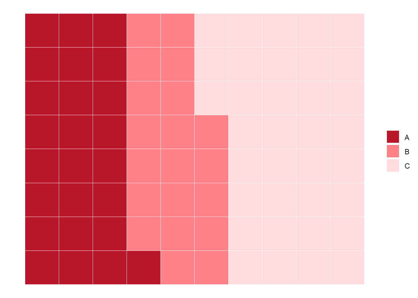
The package ggpol offers an interesting visualization in the shape of
a array of “seats” in a parliament. ( There is also a package called
ggparliament which in my opinion is a bit cumbersome, having a two
step procedure to convert data into “parliament form” etc. )
df <- data.frame(group = LETTERS[1:3],
                 value = c(25, 20, 35))

# Parliament Plot
ggplot(df) +
  ggpol::geom_parliament(aes(seats = value,
                             fill = group),
                         r0 = 2, # inner radius
                         r1 = 4 # Outer radius
  ) +
  scale_fill_manual(name = NULL,
                    values = c("#BA182A", "#FF8288", "#FFDBDD"),
                    labels = c("A", "B", "C")) +
  coord_equal() +
  theme_void()
## Warning: Using the `size` aesthetic in this geom was deprecated in ggplot2 3.4.0.
## ℹ Please use `linewidth` in the `default_aes` field and elsewhere instead.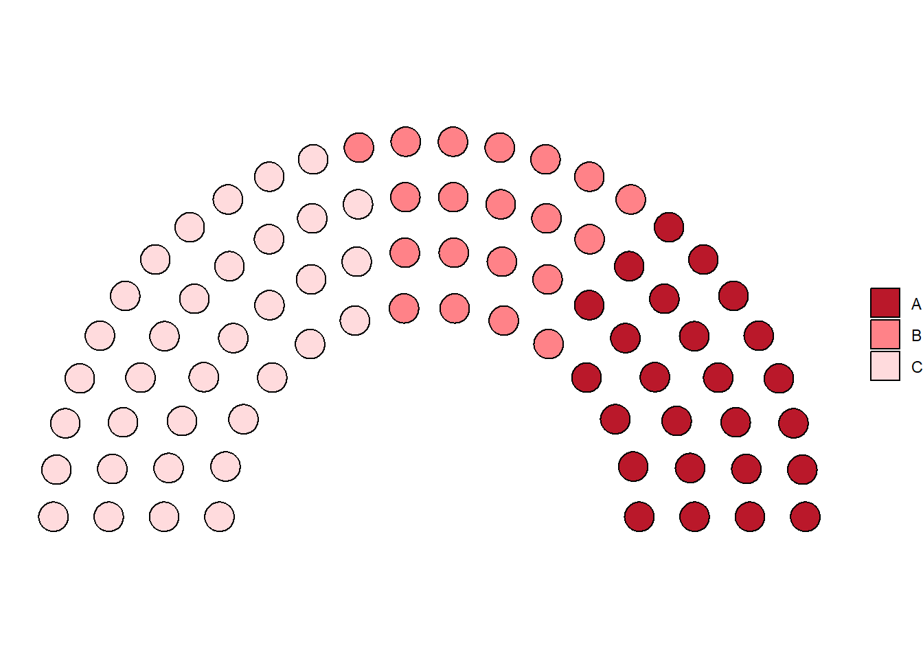
Trees, Dendrograms, and Circle Packings
There are still more esoteric plots to explore, if you are hell-bent on
startling people ! There is an R package called ggraph, that can do
these charts, and many more:
ggraph is an extension of
ggplot2aimed at supporting relational data structures such as networks, graphs, and trees. While it builds upon the foundation ofggplot2and its API it comes with its own self-contained set of geoms, facets, etc., as well as adding the concept of layouts to the grammar.
We will explore these charts when we examine network diagrams. For
now, we can quickly see what these diagrams look like. Although the
R-code is visible to you, it may not make sense at the moment!
Dendrograms
From the R Graph Gallery Website :
Dendrograms can be built from:
Hierarchical dataset: think about a CEO managing team leads managing employees and so on.
Clustering result: clustering divides a set of individuals in group according to their similarity. Its result can be visualized as a tree.
# create an edge list data frame giving the hierarchical structure of your individuals
d1 <- data.frame(from="origin", to=paste("group", seq(1,5), sep=""))
d2 <- data.frame(from=rep(d1$to, each=5), to=paste("subgroup", seq(1,25), sep="_"))
edges <- rbind(d1, d2)

# Create a graph object
mygraph1 <- tidygraph::as_tbl_graph( edges )

# Basic tree
p1 <- ggraph(mygraph1, layout = 'dendrogram', circular = TRUE) +
  geom_edge_diagonal() +
  geom_node_point() +
  theme_void()


# create a data frame
data <- data.frame(
  level1="CEO",
  level2=c( rep("boss1",4), rep("boss2",4)),
  level3=paste0("mister_", letters[1:8])
)

# transform it to a edge list!
edges_level1_2 <- data %>% select(level1, level2) %>% unique %>% rename(from=level1, to=level2)
edges_level2_3 <- data %>% select(level2, level3) %>% unique %>% rename(from=level2, to=level3)
edge_list=rbind(edges_level1_2, edges_level2_3)

# Now we can plot that
mygraph2 <- as_tbl_graph( edge_list )
p2 <- ggraph(mygraph2, layout = 'dendrogram', circular = FALSE) +
  geom_edge_diagonal() +
  geom_node_point() +
  theme_void()

p1 + p2+ theme(aspect.ratio = 1)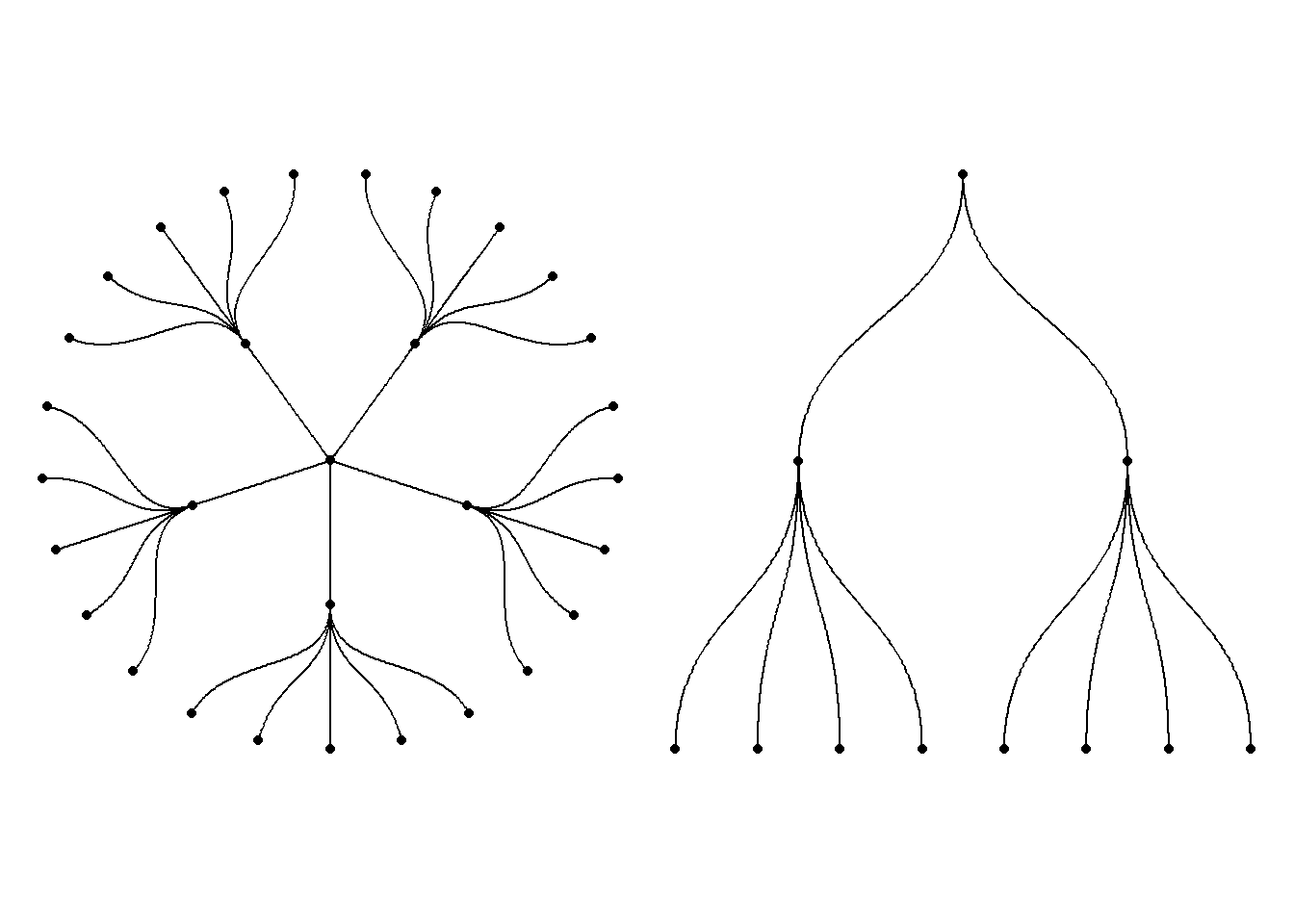
Circle Packing
library(tidygraph)
library(ggraph)
graph <- tbl_graph(flare$vertices, flare$edges)
set.seed(1)
ggraph(graph, 'circlepack', weight = size) +
  geom_node_circle(aes(fill = as_factor(depth)), size = 0.25, n = 50) +
  coord_fixed() +
  scale_fill_discrete(name = "Depth") +
  theme_void()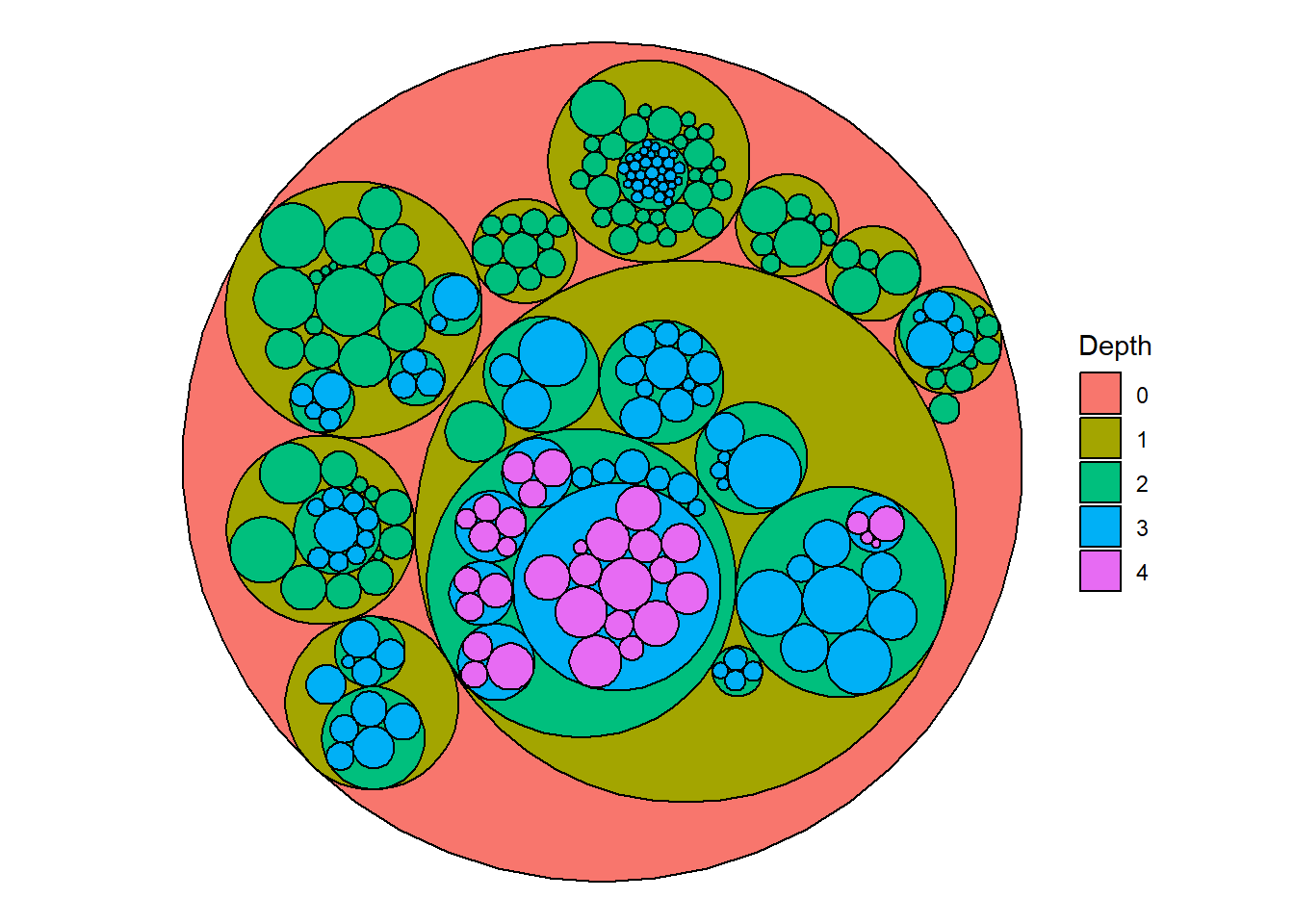
Your Turn
- Use the
penguinsdataset from thepalmerpenguinspackage and plot pies, fans, and donuts as appropriate. - Look at the
whigsandhighschooldatasets in the packageggraph. Plot Trees, Dendrograms, and Circle Packings as appropriate for these.
References
ggpolGuide by Frederik Tiedemann, https://erocoar.github.io/ggpol/Thomas Lin Pedersen,
ggraph:A grammar of graphics for relational data, https://ggraph.data-imaginist.com/Venn Diagrams in R, Venn diagram in ggplot2 | R CHARTS (r-charts.com)
EagerEyes.Org. https://eagereyes.org/pie-charts https://eagereyes.org/pie-charthttps://eagereyes.org/pie-chart
Arvind V.
My research interests are Complexity Science, Creativity and Innovation, Problem Solving with TRIZ, Literature, Indian Classical Music, and Computing with R.